Designer Background
Table of contents
- DWI Denoising with MPPCA
- DWI Gibbs Correction
- Rician bias correction
- EPI distortion correction and Eddy current and motion correction
- b0 normalization
- b1 inhomogeneity correction
- Preprocessing data with multiple diffusion encodings (b-tensor shapes) and echo times - (eddy_fakeb option)
For most single/multi-shell diffusion weighted imaging data, we recommend running designer using the following preprocessing methods. We summarize and provide references for the methods below. For their usage in Designer please see the usage page.
DWI Denoising with MPPCA
Designer includes the -denoise optional argument, which implements dMRI noise level estimation and denoising based on random matrix theory. The method exploits data redundancy in the patch-level PCA domain (Veraart2016b, CorderoGrande2019, Olesen2022). The method uses the prior knowledge that the eigenspectrum of random covariance matrices is described by the universal Marchenko-Pastur (MP) distribution.
The method used in Designer contains additional functionality compared to the original implementation. This includes adaptive patching, eigenvalue shrinkage, a modified threshold on the principal component domain, and eigenvalue shrinkage.
Adaptive patching
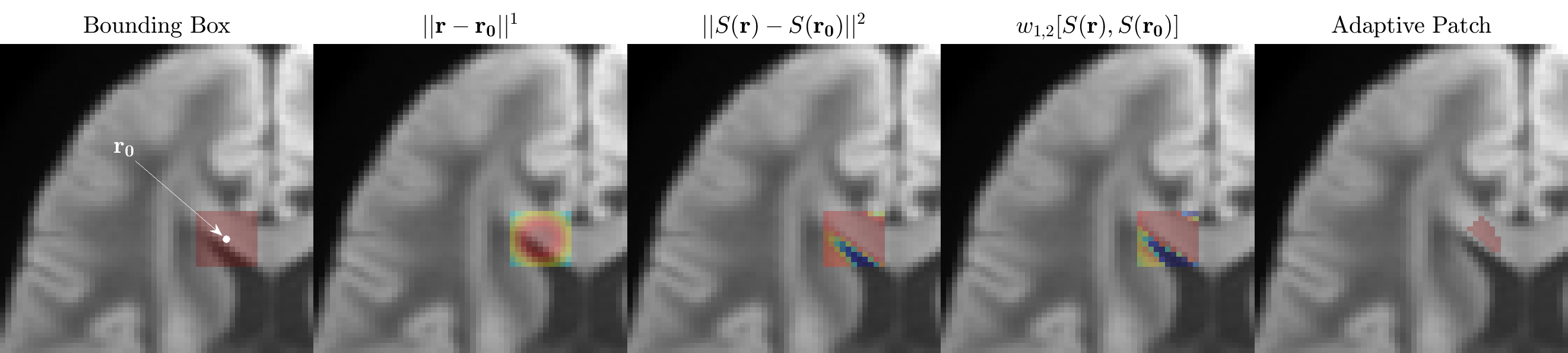
In contrast to the original MPPCA approach where patches are squares or cubes around a given voxel (e.g., $5\times5\times5$ voxels), we enhanced the spatial redundancy, in addition to the redundancy in the measurements (here in the diffusion $q$-space), by pre-selecting voxels that have similar ground truth. Our goal is to minimize the number $p$ of components, and to maximize their contributions $s_i$, such that they describe most of the signal — this is the assumption of the underlying noise-free signal to be of low-rank.
Hence, for a voxel at $\br_0$, we would like to include the signals $S_m(\br_n)$ such that both $S_m$ are close to each other for different $\br_n$, and the voxels $\br_n$ are not too far from $\br_0$. The “distance” between signals can be described as: $w_{\alpha,\beta}[S(\br), S(\br’)] = |\br -\br’|^\alpha \cdot |S(\br)-S(\br’)|^\beta$.
Here, $|\br -\br’|$ is the Euclidean distance between voxels in 3 dimensions, and $|S(\br)-S(\br’)| = \sqrt{\sum_m |S_m(\br) - S_m(\br’)|^2}$ is the Euclidean distance between signals (the norm over the measurement index $m$).
The balance of preferring the distance between voxels and between signals is tuned by the choice of exponents $\alpha$ and $\beta$. Here we choose $\alpha=1$ and $\beta=2$ based on an empirical observation of improved denoising performance when $\beta > \alpha$ (preferring similarity of signals to the distance from $\br_0$). When $\alpha \gg \beta$ this method converges to the original MPPCA patching implementation (local signal-independent patch around $\br_0$). Based on the above distance function, we choose a patch around voxel at $\br_0$ as $N$ voxels (including $\br_0$), for which $w_{1,2}[S(\br_n), S(\br_0)]$ is the smallest. In Designer $N$ is 100 by default.
Symmetric PCA Thresholding
A data matrix $X = {X_{mn} } \equiv { S_m ( \br_n ) }$ of size $M\times N$ is formed by $M$ measurements from $N$ voxels in a patch. Let $M’ = \min(M,N)$ and $N’ = \max(M,N)$. Low-rank denoising corresponds to keeping $p$ largest components in the SVD of $X=\sum_{i=1}^{M’} s_i u_i\otimes v_i$, where $u_i$ and $v_i$ are the left and right singular vectors.
For the pure-noise case of $p=0$, all components of $XX^\top$ form the MP distribution, which has two independent properties: $\sigma^2 = \sum x_i /(MN)$, and $\sigma^2 = (x_i-x_{M’})/4\sqrt{MN}$. MPPCA uses these two properties to define two functions $\sigma_{1,2}(p)$ accounting for the noise variance from the bottom $M’-p$ components, with $p$ being the solution for $\sigma_1(p)=\sigma_2(p)$. Here, we use the following definitions based on considerations from Olesen et al..
\[\begin{align} \sigma_1^2(p) &= \frac{1}{(N'-p)(M'-p)}\sum_{i=p+1}^{M'} x_i \\\\ \sigma_2^2(p) &= \frac{x_{p+1}-x_{M'}}{4\sqrt{(N'-p)(M'-p)}} \end{align}\]These are symmetric in $M’$ and $N’$, whereas the original MPPCA formulation had $N’$ instead of $N’-p$.
Singular Value Shrinkage
To overcome the eigenvalue repulsion due to noisy components, we reduce the sample singular values $s_i$ when recombining selected principal components into a low-rank matrix $\hat{X_\eta} = \sqrt{M’}\sigma \sum_{i=1}^p\, \eta(s_i/(\sqrt{M’}\sigma))\, u_i \otimes v_i$. According to Gavish et al., the optimal shrinker function based on minimizing MSE of the Frobenius norm can be expressed as
\[\eta(s) = \begin{cases} \frac{1}{s}\sqrt{(s^2-\gamma-1)^2-4\gamma} & s > 1 + \sqrt{\gamma} \,, \\ \\ 0 & s \leq 1 + \sqrt{\gamma} \,, \end{cases}\]where $\gamma = M’/N’\leq 1$.
\[p(\lambda) = \begin{cases} \frac{\sqrt{(\lambda-\lambda_{-})(\lambda_{+}-\lambda)}}{2\pi\lambda\sigma^2(M/N)} & \lambda_{-}<\lambda<\lambda_{+} \,, \\ \\ 0 & \text{otherwise} \end{cases}\]Denoising Complex Data
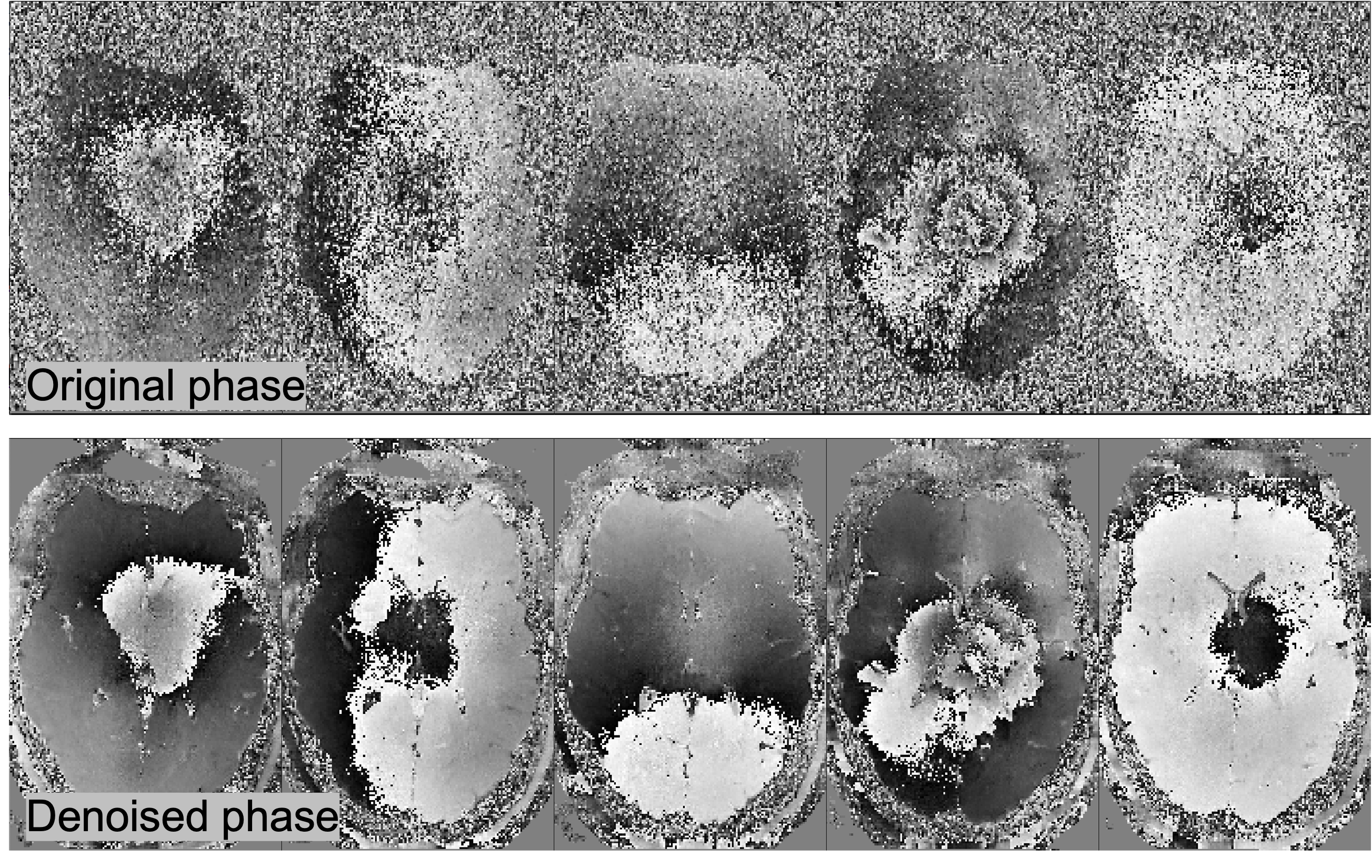 Designer provides users with the option to include a phase dataset as an optional input. To perform denoising on complex data, Designer first denoises the complex data using MPPCA (symmetric thresholding) using a $15 \times 15$ 2d box-shaped kernel within each slice. The denoised and spatially smoothly-varying phase $\phi_{\rm dn}(\br)$ is then unwound according to: $S_{\rm real} = $Re$\,(S_{\rm complex} e^{-i\phi_{\rm dn}})$. Finally, the noisy phase-unwound signal $S_{\rm real}$ is denoised using an adaptive 3d moving patch, symmetric thresholding, and eigenvalue shrinkage. Phase unwinding helps remove spurious components arising due to shot-to-shot phase variations in dMRI. In addition to improved denoising performance (due to the two-pass approach), MP-Complex also reduces the Rician noise floor of the data, reducing bias and increasing the precision of downstream parameter estimation.
DWI Gibbs Correction
This application attempts to remove Gibbs ringing artifacts from MRI images using the method of local subvoxel-shifts proposed by Kellner et al. and extended to Partial Fourier acquired images by Lee et al.. This method is designed to work on images acquired with either full k-space coverage or partial k-space coverage, by setting the input argument -pf.
The augmented pipline to eliminate 6/8 Partial Fouerier induced Gibbs ringing is shown here (reproduced from Lee et al.): 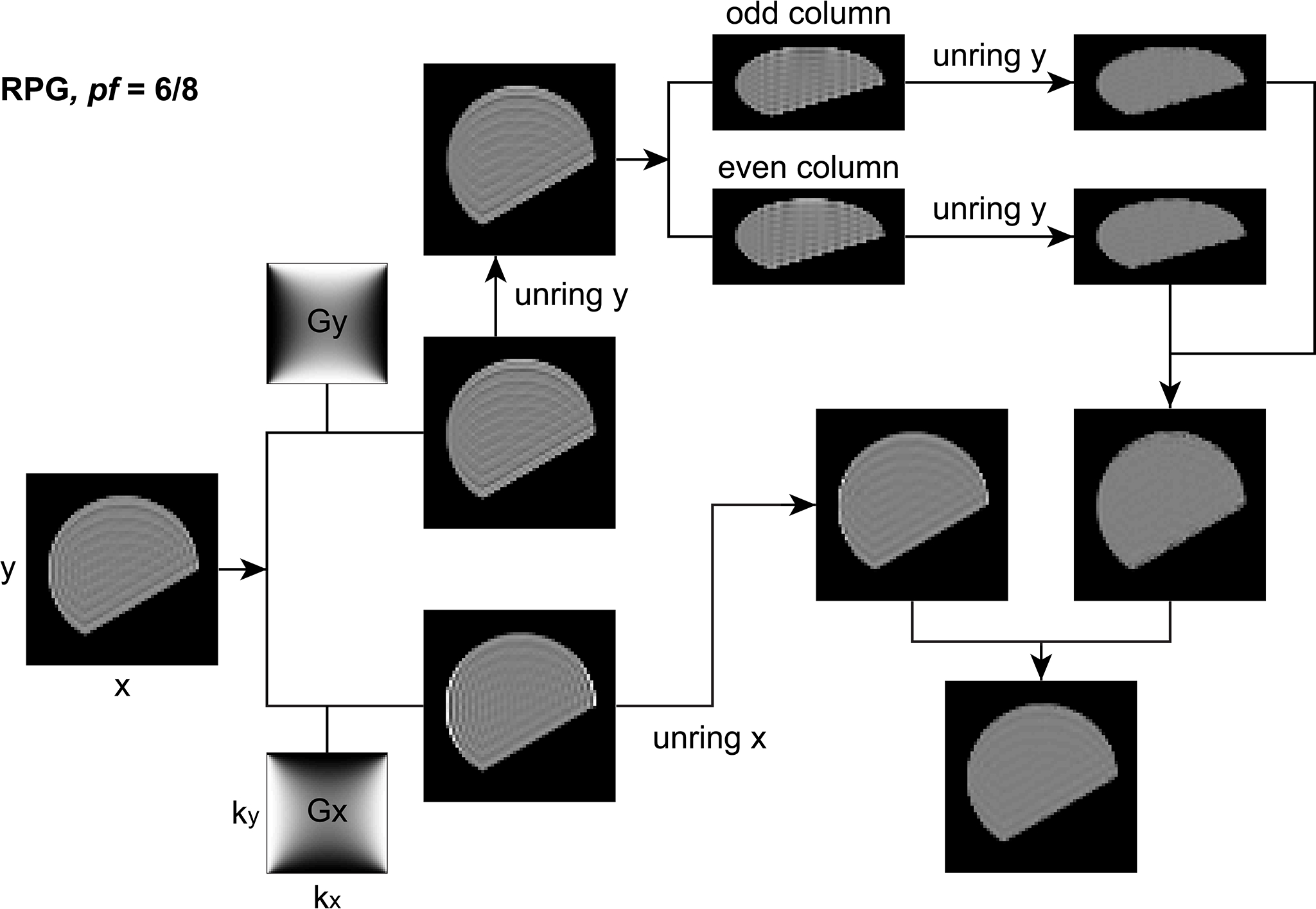 The PF acquisition and zero filling induce extra ringings of interval $2\Delta y$ in phase-encoding (y) direction. The ringing removal pipeline has two steps: First, the weighting filter $Gy$ is applied to the Fourier domain of the original image, smoothing out ringings of interval $\Delta x$ in x-direction. The remaining ringings of interval $\Delta y$ in y direction are subsequently removed by applying unring y to the image, and ringings of interval $2\Delta y$ are removed by applying unring y to sub-images consisting of odd columns and even columns respectively. Combining the two sub-images, we obtain the first corrected image. Secondly, the weighting filter $Gx$ is applied to the Fourier domain of the original image, smoothing out ringings of interval $\Delta y$ in y direction. The remaining ringings of interval $\Delta x$ in x direction are further removed by applying unring x to the image, and ringings of interval $2 \Delta y$ in y direction are kept untreated. Then we obtain the second corrected image. Finally, the average of two corrected images yields the output image. In this figure, each image is rotated by 90$\circ$, and the column in each image is in a horizontal direction.
Phantom example of PF induced gibbs: 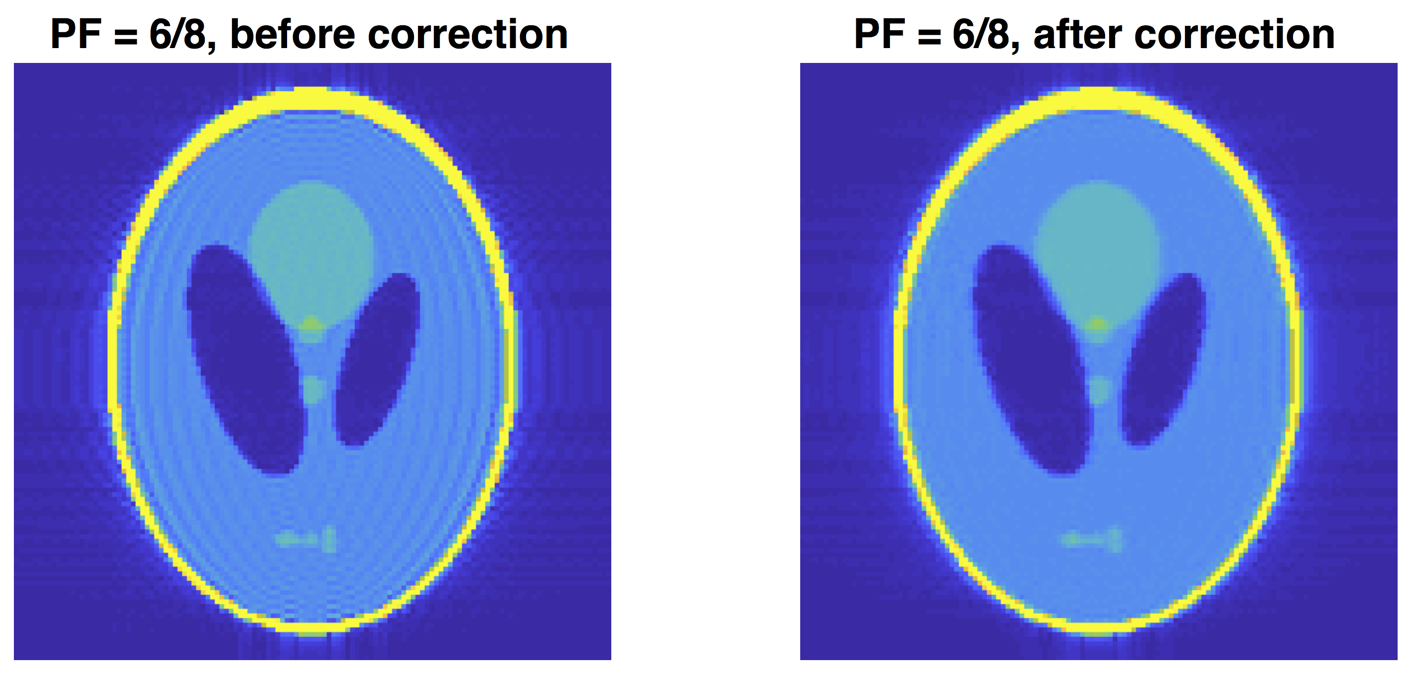
Rician bias correction
In addition to high noise levels inherent to MRI, noise in DICOM level MRI data (data that has gone through a standard reconstruction from k-space to image space) is no longer Gaussian in profile. Since MRI data is acquired in the frequency (k-space) domain it comes with two noise channels, a real noise channel and an imaginary noise channel. DICOM level MRI data consists of the absolute value of this complex information, which means that the Gaussian noise inherent to the raw data becomes skewed during image reconstruction. The image below shows the process of how signal and noise skew in the positive direction during reconstruction. This positive bias will also bias quantitative scalar maps. 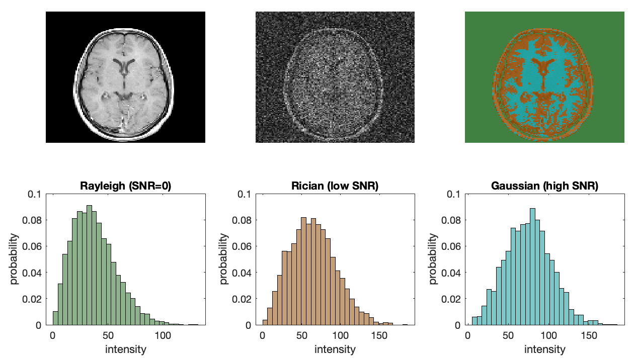
Designer offers two methods for the reduction of Rician bias. The first is by including the -phase option along with the -denoise option in order to perform complex denoising.
The second method is through the -rician option which uses the method of Koay et al. to approximate the level of bias using $\sigma$ estimated using MPPCA. The form of this approximate bias correction is $S’ = \sqrt{S^2 - \sigma^2}$. Where $S$ is the magnitude DWI signal.
The -rician option is designed for data with SNR > 2. If your data does not meet this criteria we strongly recommend using the -phase option for performing noise floor corrections.
EPI distortion correction and Eddy current and motion correction
Designer makes use of topup, eddy, and the mrtrix3 script dwifslpreproc, for the majority of EPI and motion correction steps. Designer encapsulates some of the surrounding image data and metadata processing steps either by parsing the BIDS json sidecar or through the use of input parameters pe_dir and -pf. It is intended to simplify these processing steps for most commonly-used DWI acquisition strategies, whilst also providing support for some more exotic acquisitions. The usage and examples sections demonstrates the ways in which the script can be used based on the (compulsory) -rpe_* command-line options, akin in the implementation of dwifslpreproc.
The script will attempt to run the CUDA version of eddy; if this does not succeed for any reason, or is not present on the system, the CPU version will be attempted instead. By default, the CUDA eddy binary found that indicates compilation against the most recent version of CUDA will be attempted; this can be over-ridden by providing a soft-link “eddy_cuda” within your path that links to the binary you wish to be executed.
Additional motion correction can be performed by using the -pre_align option, which is designed to simply align the first b0 image from each input series, such that for input series with large motion between them will be better conditioned for input to eddy.
Users can also use the command -ants_motion_correction to perform volume-to-volume rigid registrations. This option is included for cases with such severe motion or unusual gradient schemes that eddy is not enough to completely eliminate motion artifacts from the data. It should be noted that each of the options - eddy, pre_align, and -ants_motion_correction will interpolate the dwi data and these options should not all be used by default. We recommend using eddy as the default motion correction strategy and using the other two options only in cases of severe motion.
b0 normalization
Designer performs normalization in a specific manner for cases where multi-shell data is sent as separate input series. It performs voxelwise rescaling by taking the ratio of smoothed (Gaussian kernel (mm) with 3 standard deviations) b=0 images from each series to rescale all subsequent diffusion-weighted images. This is of particular importance in the case where this are changes in amplifier gain between input series, or when certain scan parameters such as “prescan normalize” are on for some series and off for others.
b1 inhomogeneity correction
Perform B1 field inhomogeneity correction for a DWI volume series using ants N4 bias field correction.
Preprocessing data with multiple diffusion encodings (b-tensor shapes) and echo times - (eddy_fakeb option)
Rationale behind the fake-b option: We have found that when running eddy, it is more robust to process all the data together rather than doing it in batches, separating scans, and registering all blocks afterwards. This is why we added this option to designer: -eddy_fakeb This is nothing more than a trick to go around eddy so that you can process multiple b-tensor encodings and variable TE data rather than having to process them in batches that are later co-registered. An example on how to do this is:
dwi1=${raw}/LTE_TE92.nii
dwi2=${raw}/PTE_TE92.nii
dwi3=${raw}/STE_TE92.nii
dwi4=${raw}/LTE_TE62.nii
dwi5=${raw}/PTE_TE80.nii
dwi6=${raw}/LTE_TE130.nii
# The above are just the filenames of your magnitude data (if you have their corresponding phase maps you can use them too)

designer \
-denoise -degibbs \
-pre_align -ants_motion_correction \
-eddy -rpe_pair rpe_b0.nii -rpe_te 62 -pe_dir AP \
-echo_time 92,92,92,62,78,130 \
-bshape 1,-0.5,0,1,-0.5,1 \
-eddy_groups 1,2,3,4,5,6 \
-normalize -mask \
-scratch designer_processing_variable_te_beta -nocleanup \
$dwi1,$dwi2,$dwi3,$dwi4,$dwi5,$dwi6 dwi_designer.mif
Note that now you need to specify the b-tensor shape and TE of each scan. If you acquired phase maps, you can also perform complex MPPCA denoising. This -eddy_fakeb option allows us to trick eddy into processing all shells together. Thus, there should be less residual motion after designer now. In many ‘good’ subjects, this performs identically to running eddy in different groups and then registering the groups but in some more challenging cases, this change improves things. The ‘fake b-value’ option is just a multiplication factor that artificially changes the b-value of some scans such that eddy treats a given shell as a higher diffusion weighting. This is done so that b=2000 s/mm^2 LTE and b=2000 s/mm^2 PTE are not merged in eddy (we know they are different but eddy, whose only inputs are bvals and bvecs, does not know). For example, if you focus on the TE92 subset of this protocol, you have (in s/mm^2):
- LTE: b=1000, b=2000, b=6000.
- PTE: b=0, b=2000.
- STE: b=0, b=1500. (note all b0s are identical measurements since there is no diffusion encoding so there is no such thing as an LTE/PTE/STE b0)
Thus, based on the b-values above eddy will not merge LTE and STE since these shells differ on b-value. However, eddy will mix the two b=2000 shells in its processing and this will introduce biases because the contrast differs between these images. To make sure eddy treats LTE b=2000 and PTE b=2000 sets of DWIs separately, we tell eddy that the b-value of the PTE shell is 2000*1.4=2800 and thus, treats it as an independent shell. After eddy, we replace the fake b-value with the original one.
The above trick works because eddy makes very few assumptions about the data and the relations between directions of different shells. It is a workaround to not have to rewrite eddy and make it detect non-LTE encodings (eddy was conceived to process only LTE data, but the assumption of a Gaussian process holds for any b-tensor shape). Note that if all your data has the same bandwidth, you can get away with acquiring a single b0 with reverse phase encoding (rather than one per TE). We use the input rpe_b0.nii and its corresponding b0 to compute distortions with topup and then applied these deformations to all datasets.