Diffusion Tensor and Kurtosis Tensor Representations
Table of contents
This page describes background on how the diffusion and kurtosis tensors are fit in TMI. For information on the particular DTI/DKI fitting options available with TMI please see the usage page.
The Basics
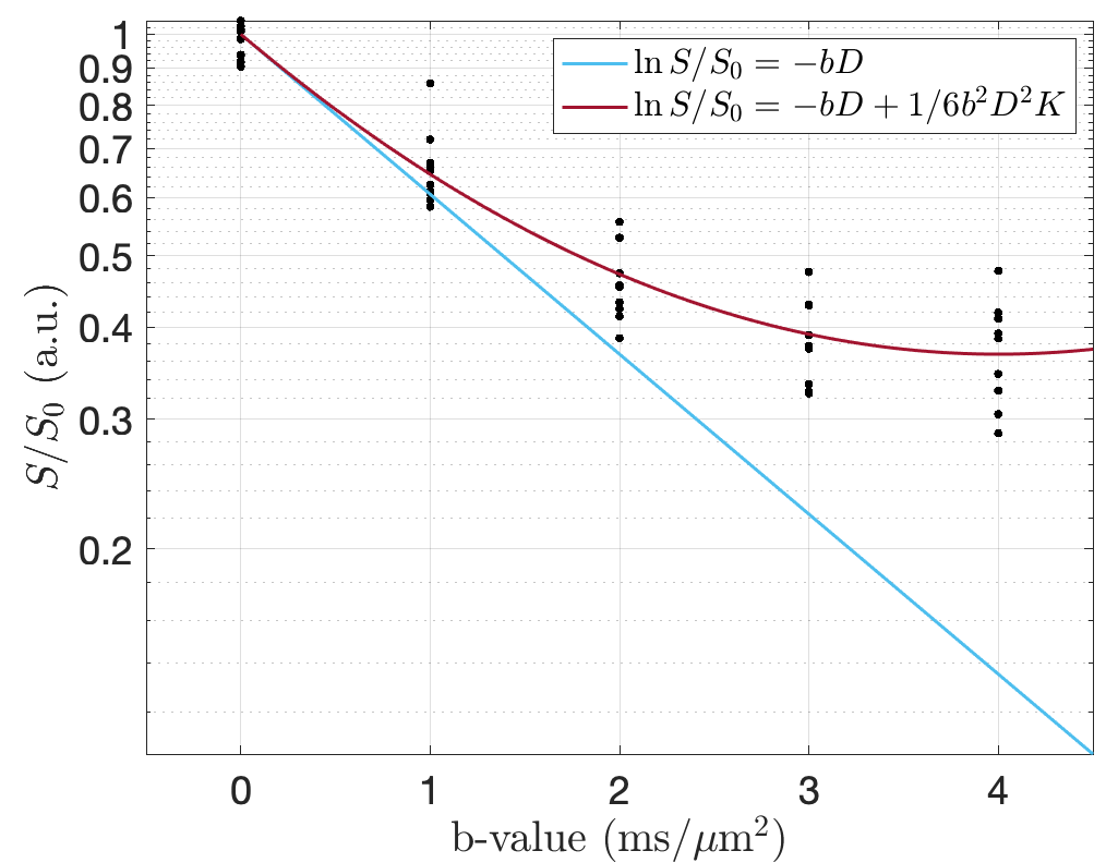
We can expand the signal in powers of the applied gradient in order to reflect the diffusion properties of a given medium. This allows us to compliment the diffusion coefficient which approximates free diffusion with an infinite series of other parameters that add complexity to the behavior of spin phases. The cumulant expansion of the diffusion signal for a Gaussian propagator simplifies to $S = S_0 e^{-bD}$, where $b$ refers to the b-value. For non-Gaussian diffusion we can include more signal cumulants in the expansion, i.e. $S = S_0 e^{-bD + O(b^2)} = S_0 e^{-bD + 1/6 D^2 b^2 W + O(b^4)}$.
In tissue, we cannot expect axons to line up perfectly with applied gradient fields. If we want to effectively measure diffusion in tissue with many orientations, we must also sample along many gradient directions. We can express $b$, $D$, and $K$, in the above expression as tensors, and use the eigenvalues of $D$ and $K$ to measure the amount of diffusion or kurtosis in each direction. For diffusion tensor imaging (DTI), as least 6 unique gradient directions are required, and for higher order diffusion schemes such as diffusion kurtosis imaging (DKI), at least 15 additional directions must be acquired. In practice, precision requirements demand closer to 30 directions for DTI and 90 for DKI to reach sufficient data quality for practical use.
The Diffusion and Kurtosis Tensors
The image above shows diffusion MRI signal attenuation as a function of diffusion weighting. The blue curve shows the diffusion tensor imaging representation, where only a single non-zero b-value is needed to estimate the linear function. This curve shows only estimated mean diffusion, however in diffusion tensor imaging, $D$ is a tensor whose eigenvalues represent the magnitude of diffusion in each direction.
We solve for $D$ using lease squares according to $X = BD$, where $X$ $ =\ln(S/S_0)$. Therefore with exactly 6 directions $D=B^{−1}X$, or $D = (B^{\top}B)^{−1}B^{\top}X$ (classical LLS estimator) with more than 6 directions. The linear least squares method is the simplest solution to computing the diffusion tensor. In practice, TMI performs weighted linear least squares (WLLS), where we perform two fit iterations. First the diffusion tensor is fitted to the log-signal using LLS where all measurements contribute equally to the fit, then the fit is iterated with weights determined by empirical signal intensities from the prior iteration step. See Veraart 2013 for more details on this fitting method.
For fitting the diffusion tensor, TMI includes only data up to b1000. If data with larger b-values are included in the input dataset, the data is truncated such that the maximum b-shell is no larger than 1000. The kurtosis tensor is fit with data up to b3000.
The tensor coefficients are stored according to the mrtrix3 convention:
DT volumes 0-5: $D_{11},D_{22},D_{33},D_{12},D_{13},D_{23}$.
KT volumes 0-2: $W_{1111},W_{2222},W_{3333}$
KT volumes 3-8: $W_{1112},W_{1113},W_{1222},W_{1333},W_{2223},W_{2333}$
KT volumes 9-11: $W_{1122},W_{1133},W_{2233}$
KT volumes 12-14: $W_{1123},W_{1223},W_{1233}$.
Tensor parameters
The eigenvalues $\lambda_1 \geq \lambda_2 \geq \lambda_3$ of $\mathbf{D}$ represent the shape of the tensor, and the corresponding eigenvectors of $\mathbf{D}$ represent the orientation of the diffusion tensor. To highlight specific features of the tensor we commonly use scalar representations including the trace ${\rm TR}(\mathbf{D}) = \lambda_1 + \lambda_2 + \lambda_3$.
The mean diffusivity (MD) is then $\frac{1}{3}\sum_{i=1}^3 \lambda_i$. We refer to axial diffusivity (AD) as the diffusion along the primary eigenvalue direction $\lambda_1$, and the radial diffusivity (RD) as the mean over eigenvalues orthogonal to the primary direction, $\frac{1}{2}(\lambda_2+\lambda_3)$.
The fractional anisotropy (FA) represents the degree of tissue dispersion and is the normalized standard deviation of eigenvalues, defined as $FA = \sqrt{\frac{1}{2}}\frac{\sqrt{(\lambda_1-\lambda_2)^2 + (\lambda_2 - \lambda_3)^2 + (\lambda_1 - \lambda_3)^2}}{\sqrt{\lambda_1^2+\lambda_2^2+\lambda_3^2}}$. We can create color FA images by scaling the principal diffusion tensor eigenvector by FA and mapping the result to an RGB colormap.
Likewise, the kurtosis tensor parameters MK, AK, and RK correspond the the kurtosis tensor as MD, AD, and RD correspond to eigenvalues of the diffusion tensor. For kurtosis, TMI offers two definitions of the tensor based on published conventions.
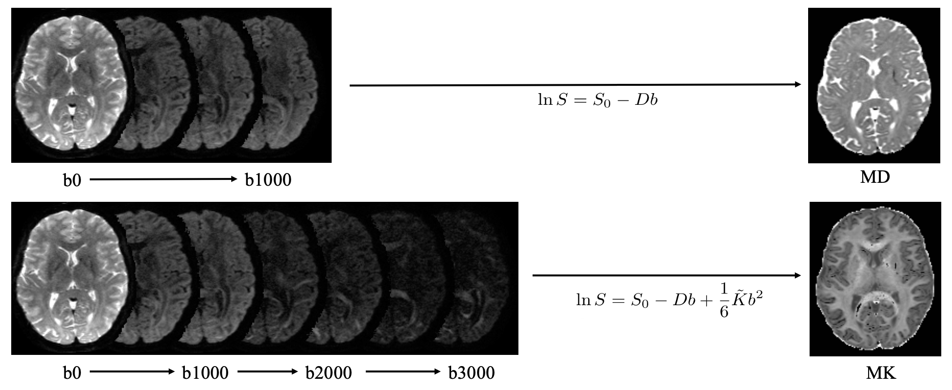 top: Simple clinical example of a mean diffusivity scalar map derived from a single b-shell acquisition Bottom: example of a mean kurtosis scalar map derived from a multi b-shell acquisition.
Outlier Detection
A simple threshold method is used to detect outliers. For each voxel, we project the kurtosis tensor along 10,000 directions and then set a threshold on the apparent kurotsis coefficient such that any((K < -1) or (K > 10)) is considered an outlier.
Outlier Replacement
Outlier replacement is performed by computing replacing each voxel detected as an outlier with the median of its non-outlier neighbors.
This can be extended to a sliding median filter, or an adaptive filtering method. This outlier replacing smoothing window is called fit _smoothing in tmi, and it runs a windowed adaptive nonlocal means filter on the dwi. For each voxel we take a cubic patch in 4d and take the mean over the n most similar voxels in xyz and q-space. n is decided by the percentile argument to tmi, where with n=10 (default) we are smoothing over the 10% most similar voxels, and so on. When you also include a map of outliers using the -akc_outliers flag, voxels that are considered outliers and ignored from a given patch. This has the effect of smooshing non outlier signal into black voxel areas. Obviously this method depends heavily on the patch size which is fixed right now.